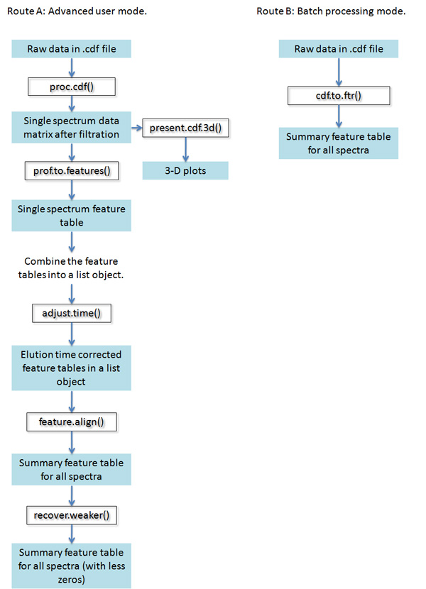
[Major steps of unsupervised analysis]

By "unsupervised" we mean analyzing the data by itself, not relying on any existing knowledge about metabolites.

Steps 1 and 2 are single spectrum procedures:

(1) From CDF format raw data, use run filter to reduce noise and select regions in the spectrum that correspond to peaks [proc.cdf()]

(2) Identify peaks from the spectrum and summarize peak location (m/z, retention time), spread and intensity [prof.to.features()]

Steps 3, 4 and 5 are multi-spectrum procedures:

(3) Retention time correction across spectra [adjust.time()]

(4) Peak alignment across spectra [feature.align()]

(5) Weak signal recovery [recover.weaker()]

The figure below summarizes the functions involved in the analysis:

The following is a demonstration with the demo dataset. All the material copied from R are in black, and all other comments are in blue.

1. Download the package and install it in R.

2. Download the data and unzip it into a folder. I am using the folder "C:/apLCMS_demo" for this demonstration.

3. Open R. Load the package.

> library(apLCMS)
Loading required package: MASS
Loading required package: rgl
Loading required package: ncdf
Loading required package: splines
Loading required package: doSNOW
Loading required package: foreach
foreach: simple, scalable parallel programming from Revolution Analytics
Use Revolution R for scalability, fault tolerance and more.
http://www.revolutionanalytics.com
Loading required package: iterators
Loading required package: snow

4. Run the analysis of the sample data using the wrapper function cdf.to.ftr(). The display from the wrapper function are mainly the names of the intermediate files being written into the folder and the processing time (in seconds). Summary and disgnostic plots (detailed below) are generated in every step. Below is a sample output.

> folder<-"C:/apLCMS_demo"
> setwd(folder)
> aligned<-cdf.to.ftr(folder, file.pattern=".cdf", n.nodes=4, min.exp=5,min.run=12,min.pres=0.5)

***************************** prifiles --> feature lists *****************************
****************************** time correction ***************************************
**** performing time correction ****
m/z tolerance level:  1.14260717038009e-05
time tolerance level: 82.5881547056058
the template is sample 8
sample 1 using 354 ,sample 2 using 409 ,sample 3 using 552 ,
sample 4 using 874 ,sample 5 using 753 ,sample 6 using 1047 ,
sample 7 using 819 ,***** correcting time, CPU time (seconds) 1.566
****************************  aligning features **************************************
**** performing feature alignment ****
m/z tolerance level:  1.14260717038009e-05
time tolerance level: 64.2255581174968
***** aligning features, CPU time (seconds): 8.571
**************************** recovering weaker signals *******************************

5. Examining the results. A list object is returned from the function. "Features" is a list of matrices, each of which is a peak table from a spectrum. "Features2" is of the same structure except the retention time is corrected. "Aligned.ftrs" is the matrix of aligned features across all the spectra. "Pk.times" is the matrix of peak retention times of the aligned features. "Final.features" is what's most important. It is the aligned feature table after weak signal recovery, i.e. the end product. "Final times" is the accompanying peak retention time matrix. A small section of the final.features table is shown. The first column of the table is the m/z value; the second column is the median retention time; from the third column on are the signal strength in each spectrum.

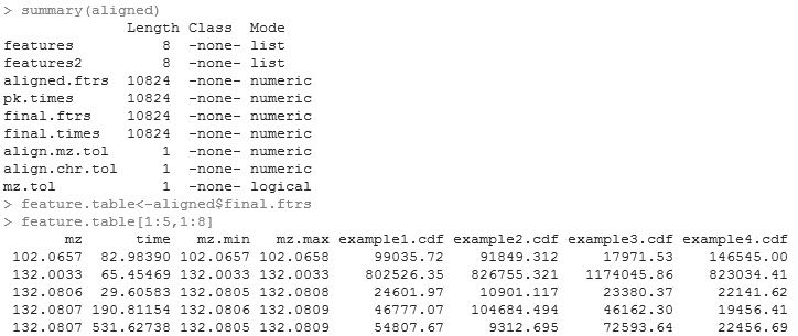
This feature table is the key output. If you prefer not to work in R for downstream analysis, you can simply output it to a tab-delimited text file, which can be read into excel and other statistical softwares easily.

> write.table(feature.table,"result.txt",sep="\t",quote=F,col.names=T, row.names=F)

Now the table file called "result.txt" is in the working directory.

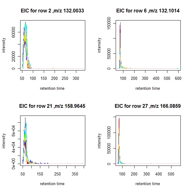
After finding some interesting features, you may want to examine the original extracted ion chromatograms of them. This can be done by using the function EIC.plot(). Here we demonstrate the usage of it by selecting some high intensity features that are present in all profiles. Notice "selection" is the rows of the feature table for which you wish to plot. It should be a vector like c(4,10,134,555).

> feature.table<-aligned$final.ftrs[,5:12]
> selection<-which(apply(feature.table!=0,1,sum)==8 & apply(feature.table,1,mean)>200000)
> EIC.plot(aligned, selection[1:4], min.run=12, min.pres=0.5)
the colors used are:
[1] "1: red" "2: blue" "3: dark blue" "4: orange" "5: green" "6: yellow"
[7] "7: cyan" "8: pink"

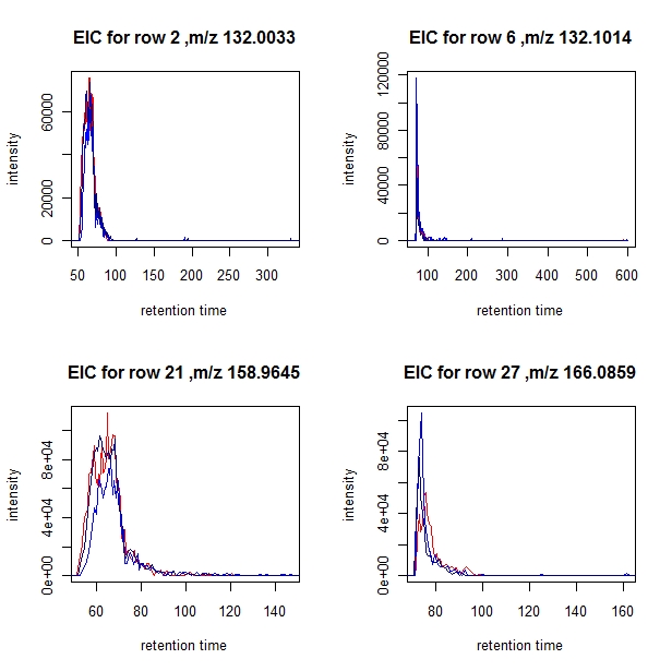
You can choose a subset of profiles for which to plot the EICs by setting a "subset" parameter. In the example below only EICs from samples 3, 6, and 8 are plotted.

> EIC.plot(aligned, selection[1:4],subset=c(3,6,8), min.run=12, min.pres=0.5)
the colors used are:
[1] "3: red" "6: blue" "8: dark blue"

------------------------------------------------------------------------

6. If you prefer not to use the wrapper, here is a demonstration of the 5 step processing.

> library(apLCMS)
> folder<-"C:/apLCMS_demo"
> setwd(folder)
> cdf.files<-dir(pattern=".cdf")
> cdf.files
[1] "example1.cdf" "example2.cdf" "example3.cdf" "example4.cdf" "example5.cdf"
[6] "example6.cdf" "example7.cdf" "example8.cdf"

6.1 Step (1), from cdf file to filtered data.

> this.spectrum<-proc.cdf(filename=cdf.files[4], min.pres = 0.5, min.run = 12, tol = 1e-5)
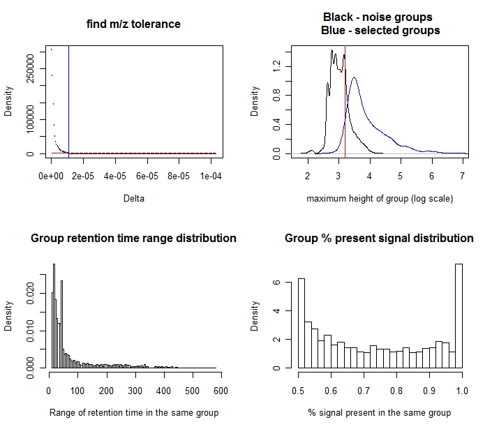
maximal height cut is automatically set at the 75th percentile of noise group heights: 1728.45823753139

> ### (and this plot is shown)

The upper-left plot is the search for the m/z tolerance.

The upper-right plot shows the distribution of the height of the signal groups. The black curve is from those groups with less intensity observations than the run filter requires (noise); the blue curve is from those passing the run filter (mostly signals). Some groups passing the run filter are eliminated because their intensities are low. The default cutoff is the redline-75th percentile from the black group. The user can input any cutoff using the parameter "baseline.correct".

The lower-left panel is the distribution of the groups' span in retention time. Because some metabolites share m/z, it is no surprise that a small number of groups have a very long span. Nonetheless the majority of the groups span <100 seconds.

The lower-right panel is the distribution of the proportion of time points where the group has an intensity observation. Because the run filter cut this value using the parameter min.pres, the minimum of the distribution is equal to min.pres. The maximum is certainly 1, where the group has no skipped time point.

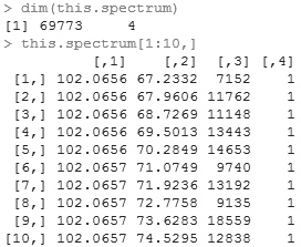
Examining the matrix, there are four columns. The first is the median m/z value of the peak,the second is the time points where the m/z is observed, the third is the signal strength at the time point, and the fourth is the group number in case two peaks share the same m/z.

We can plot the spectrum or part of it.

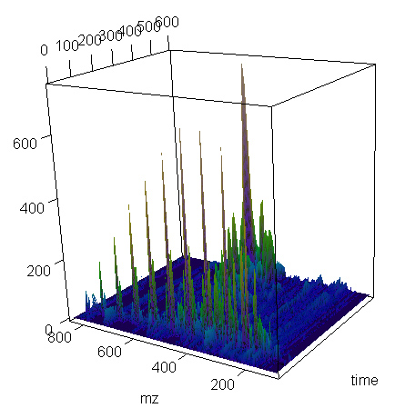
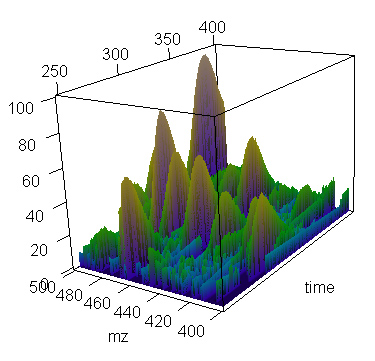
> present.cdf.3d(this.spectrum,transform="sqrt")

Notice in these plots the intensity axis is of relative scale.

> present.cdf.3d(this.spectrum,time.lim=c(250,400), mz.lim=c(400,500),transform="none")
> ### (and this plot is shown)

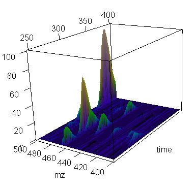
Using cube-root transform helps bring out smaller peaks.

> present.cdf.3d(this.spectrum,time.lim=c(250,400), mz.lim=c(400,500),transform="cuberoot")
> ### (and this plot is shown)

6.2 Step (2), from the filtered data to feature table of the spectrum.

> this.peak.table<-prof.to.features(this.spectrum, bandwidth = 0.5, min.bw=10, max.bw=30)

A plot is shown.

The upper-right panel is the distribution of the standard deviations of the m/z values in every feature. Notice we are using non-centroided data, which causes some spread around the true m/z. Compare this plot to the one generated by feature.align.

The lower-left panel is the distribution of the standard deviation of retention time in every feature.

The lower-right panel is the distribution of the log(peak area) of the features.

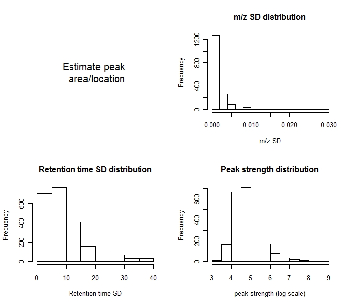
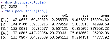
Every feature is represented by a row in this matrix. The first column is m/z, the second is retention time, the third is spread (standard deviation of the fitted normal curve), and the fourth is the estimated signal strength (peak area).

Now repeat the above step for every cdf file and obtain a list of all the peak tables. In the wrapper function this part is run in parallel. If you know how to use foreach(), replace the for loop with it, and this part is much faster.

> features<-new("list")
> for(i in 1:length(cdf.files))
+ {
+ this.spectrum<-proc.cdf(filename=cdf.files[i], min.pres = 0.5, min.run = 10, tol = 1e-5)
+ this.peak.table<-prof.to.features(this.spectrum, bandwidth = 0.5, min.bw=10, max.bw=30)
+ features[[i]]<-this.peak.table
+ }
m/z tolerance is:  1e-05
maximal height cut is automatically set at the 75th percentile of noise group heights: 1967.95020262201
m/z tolerance is:  1e-05
maximal height cut is automatically set at the 75th percentile of noise group heights: 1566.88524222241
m/z tolerance is:  1e-05
maximal height cut is automatically set at the 75th percentile of noise group heights: 1805.92912374766
m/z tolerance is:  1e-05
maximal height cut is automatically set at the 75th percentile of noise group heights: 1679.73381566848
m/z tolerance is:  1e-05
maximal height cut is automatically set at the 75th percentile of noise group heights: 1503
m/z tolerance is:  1e-05
maximal height cut is automatically set at the 75th percentile of noise group heights: 1529.99115330885
m/z tolerance is:  1e-05
maximal height cut is automatically set at the 75th percentile of noise group heights: 1805.4999307671
m/z tolerance is:  1e-05
maximal height cut is automatically set at the 75th percentile of noise group heights: 1520.24846000009

> summary(features)
     Length Class  Mode  
[1,] 10195  -none- numeric
[2,]  9955  -none- numeric
[3,] 11200  -none- numeric
[4,] 11750  -none- numeric
[5,] 11515  -none- numeric
[6,] 11450  -none- numeric
[7,] 11305  -none- numeric
[8,] 13475  -none- numeric




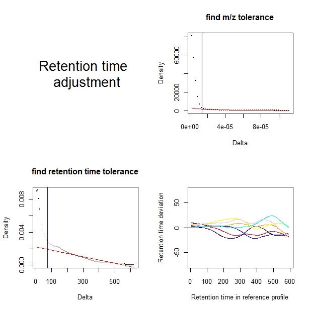
6.3 Step (3). Retention time adjustment.The procedure is based on non-parametric curve fitting. The number of features used for the curve-fitting is printed.

> features2<-adjust.time(features, mz.tol = NA, chr.tol = NA)
**** performing time correction ****
m/z tolerance level: 1.36718712335192e-05
time tolerance level: 75.532091457029
the template is sample 5
sample 1 using 566 ,sample 2 using 451 ,sample 3 using 847 ,
sample 4 using 1012 ,sample 6 using 935 ,
sample 7 using 1136 ,sample 8 using 872 ,

A plot is shown.

The upper-right panel shows the selection of m/z tolerance.

The lower-left panel shows the selection of retention time tolerance.

The lower-right panel shows the amount of adjustment for each of the profiles except the reference profile.

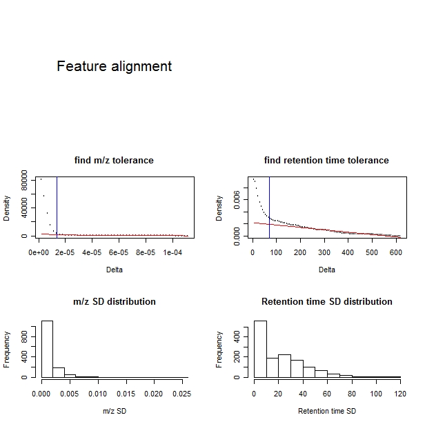
6.4 Step 4, feature alignment

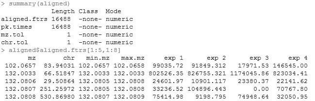
> aligned<-feature.align(features2, min.exp = 4, mz.tol = NA, chr.tol = NA)
**** performing feature alignment ****
m/z tolerance level: 1.36718712335192e-05
time tolerance level: 68.811297036486

A plot is shown.

The upper-left panel shows the selection of m/z tolerance.

The upper-right panel shows the selection of retention time tolerance.

The lower-left panel shows the distribution of the standard deviation of m/z values of the features aligned.

The lower-right panel shows ths distribution of the standard deviation of retention times of the features aligned.

6.5 Step 5, weak signal recovery.

The post.recover is the final result of the procedure. The central piece of information is the matrix post.recover$aligned.ftrs. Every row in this matrix is a feature. The first column is median m/z; the second column is median retention time; the third column is the minimum of the m/z in the profiles; the fourth column is the maximum of the m/z in the profiles; and from the fifth column on are the signal strength in each spectrum.