[Major steps of hybrid analysis]

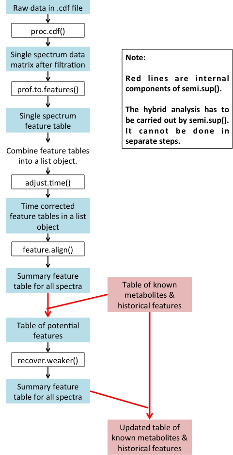
By "hybrid" we mean incorporating the knowledge of known metabolites AND/OR historically detected features on the same machinery to help detect and quantify lower-intensity peaks.

CAUTION: To use such information, especially historical data, you MUST keep using (1) the same chromatography system (otherwise the retention time will not match), and (2) the same type of samples with similar extraction technique, such as human serum.

First, it is necessary to put such information in a data frame that the program can use.

Second, the first four steps as in the unsupervised processing is conducted.

Third, the found features are merged with the data frame of known features.

Fourth, the weak signal recovery is performed using the merged feature table.

Fifth, the data frame of known metabolites and historical features is updated with the new information from the current data.

The hybrid approach is implemented in a wrapper function semi.sup(). This function carries out the above steps in a single line of command.

The figure below summarizes the hybrid procedure:

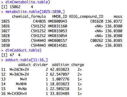
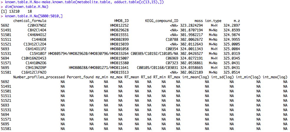
The table of known metabolites and historical features needs to be provided to the subroutine semi.sup(). The data frame is like a matrix, but different column can be different variable types. We put an example data frame in the package. The measurement variability information is NA in that data frame, because it was built from the Human Metabolome Database alone. It only contains H+ derivatives of known metabolites. After running your first batch of samples, the database will be more populated. The provided database is mainly for demonstration purposes. You can build your own database using the metabolites and ion/isotope forms of your choice.

Here's a small portion of such a table. The column names are contained in the help file of semi.sup().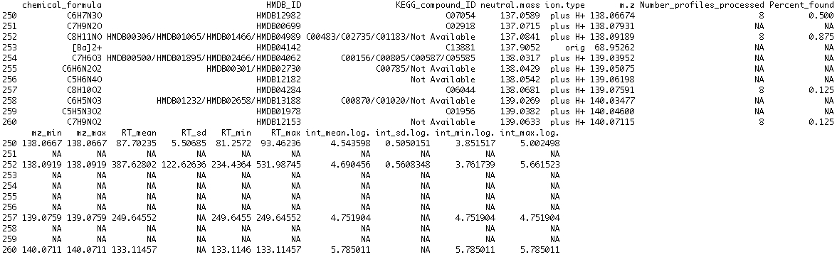

The following is a demonstration with the demo dataset. All the material copied from R are in black, and all other comments are in blue.

1. Download the package and install it in R.

2. Download the data and unzip it into a folder. I am using the folder "C:/apLCMS_demo" for this demonstration.

3. Open R. Load the package.

> library(apLCMS)
Loading required package: MASS
Loading required package: rgl
Loading required package: ncdf
Loading required package: splines
Loading required package: doSNOW
Loading required package: foreach
foreach: simple, scalable parallel programming from Revolution Analytics
Use Revolution R for scalability, fault tolerance and more.
http://www.revolutionanalytics.com
Loading required package: iterators
Loading required package: snow

4. Run the analysis of the sample data using the wrapper function semi.sup().

> folder<-"C:/apLCMS_demo"
> setwd(folder)
> data(known.table.hplus)
> aligned.hyb<-semi.sup(folder, file.pattern=".cdf", known.table=known.table.hplus, n.nodes=4, min.pres=0.5, min.run=12, mz.tol=1e-5, new.feature.min.count=4)

***************************** prifiles --> feature lists *****************************
****************************** time correction ***************************************
**** performing time correction ****
m/z tolerance level: 1.14260717038009e-05
time tolerance level: 82.5881547056058
the template is sample 8
sample 1 using 352 ,sample 2 using 410 ,sample 3 using 554 ,
sample 4 using 876 ,sample 5 using 757 ,sample 6 using 1047 ,
sample 7 using 843 ,***** correcting time, CPU time (seconds) 1.71
**************************** aligning features **************************************
**** performing feature alignment ****
m/z tolerance level: 1.14260717038009e-05
time tolerance level: 70.6474780161716
***** aligning features, CPU time (seconds): 19.913
merging to known peak table
**************************** recovering weaker signals *******************************

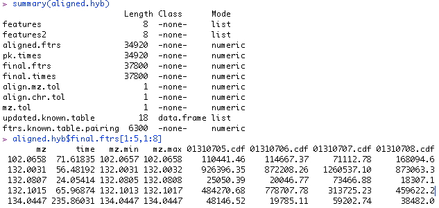
5. Examining the results. A list object is returned from the function. "Features" is a list of matrices, each of which is a peak table from a spectrum. "Features2" is of the same structure except the retention time is corrected. "Aligned.ftrs" is the matrix of aligned features across all the spectra. "Pk.times" is the matrix of peak retention times of the aligned features. "Final.features" is what's most important. It is the aligned feature table after weak signal recovery, i.e. the end product. "Final times" is the accompanying peak retention time matrix. A small section of the final.features table is shown. The first column of the table is the m/z value; the second column is the median retention time; from the third column on are the signal strength in each spectrum.

This feature table is the key output. If you prefer not to work in R for downstream analysis, you can simply output it to a tab-delimited text file, which can be read into excel and other statistical softwares easily.

> write.table(aligned.hyb$final.ftrs, "result.txt",sep="\t",quote=F,col.names=T, row.names=F)

Now the table file called "result.txt" is in the working directory.

The item "aligned.hyb$updated.known.table" is the updated known feature table. For future data analysis, you should use the updated table.

> known.table.new<-aligned.hyb$updated.known.table
> save(known.table.new, file="updated_table.bin")

In the processing of next batch of data,

> load("updated_table.bin")
> aligned.hyb<-semi.sup(......, known.table=known.table.new, .......)

Now our package contains HMDB (version 3.0) metabolites, and a table of potential adducts. You can use these two pieces of information to generate known human features based on the adducts of your choice.

The HMDB metabolite data is in the object "metabolite.table".
The adduct data is in the object "adduct.table".

> data(metabolite.table)
> data(adduct.table)

metabolite and adduct table

Example: producing a table that contains the [M+H]+ and [M+Na]+ ions of all metabolites (this takes a little while because we need to merge all metabolites sharing molecular composition)

known table gen example.jpg

Then this table can be used in semi.sup() as the known.table argument.