LESSON 12

SIMPLE ANALYSES

12-1 Statistical Inference for Simple Analyses

WHAT IS SIMPLE ANALYSIS?

Examples described previously:

· Measure of effect computed in each study to estimate EÞD relationship

· Each estimate based on sample data. If a different sample drawn, different estimates would have been calculated.

· These estimates are called point estimates - each represents a single value from a range of values that might have been obtained with different samples.

What can we say about the population parameter based on the estimated parameter?

· Determine if there is evidence from the sample that the population RR, OR, or IDR estimated differs from the null value - hypothesis testing.

· May want to determine the precision of the point estimate to account for sampling variability - interval estimation.

Methods to achieve these objectives comprise the subject matter statistical inference.

STATISTICAL INFERENCES – A REVIEW

Statistical Inference Overview

Data from an incident in which a group of persons were at risk of dying.

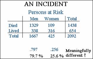
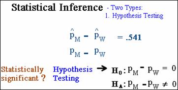
Difference in risks for men and women statistically significant?

· If we wish to draw conclusions about a population from a sample, must consider statistical inference.

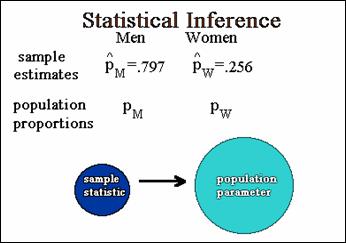
· View the 2 proportions as estimates obtained from a sample.

· The 2 sample proportions are denoted & .

· Corresponding population proportions are denoted & , without “hats”.

· Want to compare the proportions for males and females

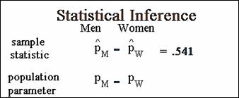
· Could use the difference between the two population proportions.

· The sample statistic is the difference between the two estimated proportions.

Hypothesis testing – difference between proportions statistically significant?

· null hypothesis – no difference between groups

· alternative hypothesis - there is a difference between the groups

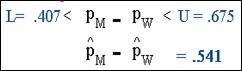
· Use interval estimation to determine precision of point estimate.

· Use sample information to compute L and U which define a confidence interval for the difference between the 2 population proportions.

· Using a confidence interval, can predict with a certain level of confidence, usually 95%, that the limits, L and U, bound the true value.

· For example data, the limits for the difference in proportions are .407 and .675, respectively.

The range of values specified by the interval takes into account the unreliability of the point estimate.

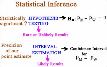
In general, interval estimation and hypothesis testing can be contrasted by differing approaches to answering questions.

· Test of hypothesis arrives at an answer by looking for unlikely sample results.

· An interval estimate arrives at its answer by looking at the most likely results, i.e., values that we are confident lie close to the parameter under investigation.

The Incident

The Titanic.

12-2 Statistical Inference for Simple Analyses (continued)

Hypothesis Testing, Part 1

Test of hypotheses, also called a test of significance

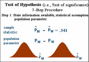
Seven-step procedure.

· Step one - state info available, statistical assumptions, and population parameter.

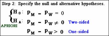
· Step 2, specify null & alternative hypotheses. H₀ is treated like the defendant in a trial - assumed true (innocent) unless evidence makes it unlikely to have occurred by chance. Null & alternative hypothesis should be made without looking at the data and based on a priori objectives of the study.

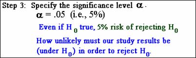
· Step 3, specify significance level, alpha. An alpha of 5% means that, if the null hypothesis is actually true, there is a 5% chance of rejecting it.

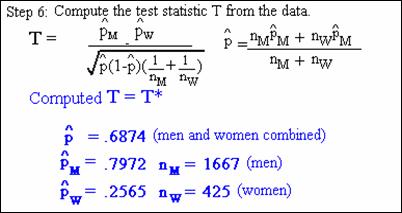
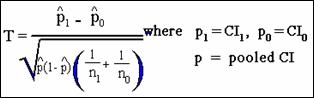
· Step 4, select test statistic; must state its sampling distribution under the assumption null hypothesis is true. Because the parameter of interest (in example) is the difference between two proportions, the test statistic T is used:

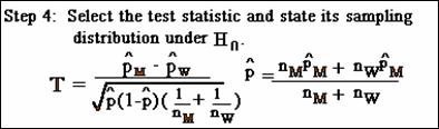
The sampling distribution of this test statistic is approximately the standard normal distribution, with mean=0 and standard deviation=1, under the null hypothesis.

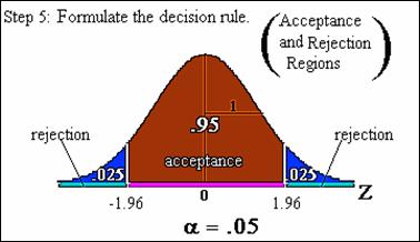
· Step 5, formulate decision rule into acceptance and rejection regions. Because the test statistic has approximately Z distribution under the null hypothesis, the acceptance and rejection regions are specified as intervals along the Z-axis.

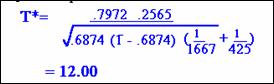
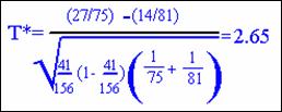
· Step 6 requires computation of the test statistic T from the observed data called T*. Here again are the sample results:

· Step 7, use computed test statistic to draw conclusions about test of significance. In this example, the computed test statistic falls into the extreme right tail of rejection region.

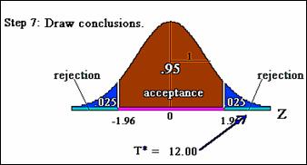
Consequently, reject null hypothesis and conclude a statistically significant difference between the two proportions at the .05 significance level.

Hypothesis Testing – The P-value

Exactly how unlikely or rare were the observed results given the null hypothesis in Titanic example?

The answer is given by the P-value. The P-value gives the probability of obtaining the value of the test statistic or a more extreme value if the null hypothesis is true.

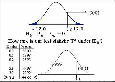
p < .0001

Confidence Intervals Review

Confidence Interval for Comparing Two Proportions

· Calculate a confidence interval for the difference proportions.

· Compute two numbers, L and U, about which we are confident, usually 95%, which surround the true value of the parameter.

· Formula for this 95 percent confidence interval:

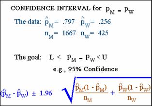
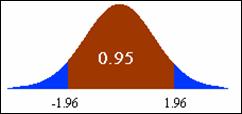
· The value 1.96 is chosen because the area between -1.96 and +1.96 under the normal curve is .95, corresponding to the 95% confidence level.

· The normal distribution is used here because the difference in the two sample proportions has approximately the normal distribution if the sample sizes in both groups are reasonably large. This is why the confidence interval formula described here is often referred to as a large-sample confidence interval.

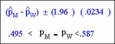
We can calculate the confidence interval for our data by substituting into the formula:

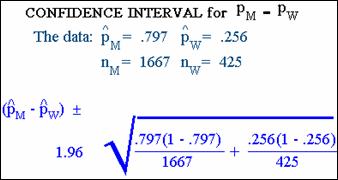
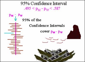
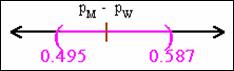
The 95% interval is .495 and .587, respectively.

Interpretation of a Confidence Interval

· How do we interpret this confidence interval?

· Consider what might happen if we were able to repeat the study, e.g., the sailing and sinking of the Titanic, several times.

· If we computed 95 percent confidence intervals for each repeat, we would expect that about 95 percent of these CIS would capture the true population difference.

Equivalent to saying that there is a probability of .95 that the interval between .495 and .587 includes the true population difference in proportions.

The true difference might actually lie outside this interval (only a 5% chance).

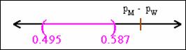
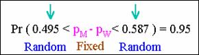
The parameter P_M – P_W does not vary at all; it is a single fixed population value. The random elements of the interval are the limits 0.495 and .587, computed from the sample data and will vary from sample to sample.

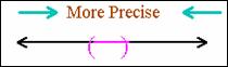
A confidence interval is a measure of the precision of an estimate

· The narrower the width of the confidence interval, the more precise the estimate.

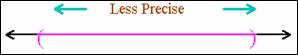
· In contrast, the wider the width is, the less precise the estimate.

COHORT STUDIES INVOLVING RISK RATIOS

Hypothesis Testing for Simple Analysis in Cohort Studies

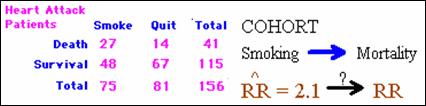
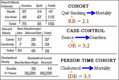
· Cohort study assessing whether quitting smoking and heart attack.

· Effect measure was the RR with an estimate of 2.1.

· What can we say about the population RR based on the sample RR?

· Is there evidence from the sample that the RR is statistically different from null?

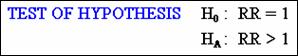
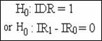
· A test of hypothesis to see if the risk ratio is significantly different from 1.

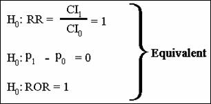
Test statistic is as follows:

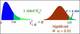
The computed value in this example of the test statistic is 2.65 with a p-value of .004; reject null hypothesis and conclude RR is significantly > 1.

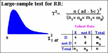
Chi Square Version of the Large-sample Test

The large-sample test for a RR can be carried out using the normal distribution or chi square (c²) distribution. The reason for this equivalence is that a standard normal variable Z squared is Z² which has a c²distribution with 1 degree of freedom.

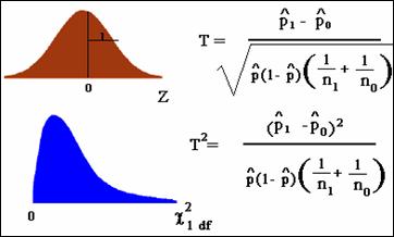
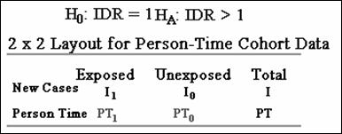
Can rewrite the statistic in terms of the cell frequencies a, b, c and d of the general 2 by 2 table:

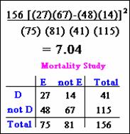
For the mortality study of heart attack, the values are c² =7.04. This value is the square of the computed test statistic we found earlier (2.65² » 7.04)

Is the c² test significant? The normal distribution version was significant at the .01 significance level, so the c² had better be significant.

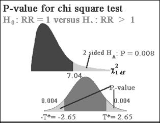
Differences between Z and c²? c² is always two-sided.

If you want to perform a 1-sided test, use normal distribution or use c² divided by 2.

The P-value for a One-Sided Chi Square Test

Not important for our class – bottom line, to compute a one-sided p-value from a chi-square test, divide the chi-square p-value by 2.

Testing When Sample Sizes Are Small

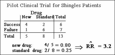
Example of small sample size: Randomized clinical trial comparing new anti-viral drug for shingles to standard drug “Valtrex”.

· Only 13 patients in the trial

· Estimated risk ratio = 3.2 - new drug was 3.2 times more successful.

Statistically significant?

· With “sparse” data / small sample sizes, use Fisher’s exact test.

· In this example, Fisher exact one-sided p-value = .0863

· Fail to reject null hypothesis (i.e., RR = 1)

COHORT STUDIES INVOLVING RISK RATIOS (continued)

Large-sample version of Fisher's Exact Test - The Mantel-Haenszel Test

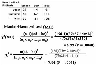
Another chi-square test used frequently in epidemiology is the Mantel-Haenszel test; works a little better than standard chi-square with sparse data:

Could use Fisher’s; one-sided p-value = .0053

All lead to the same conclusion – reject the null hypothesis

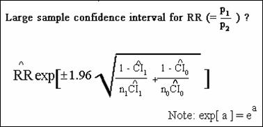
Large-Sample Confidence Interval for a Risk Ratio

More complicated than risk difference described previously.

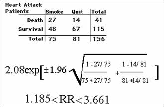
Study Question (Q12.12)

1. Interpret the above results. Does not include null …

Quiz (12.13) Do Not Worry about these questions

Calculating Sample Size for Clinical Trials and Cohort Studies

I will not ask questions concerning sample sizes on an exam.

12-6 Simple Analyses (continued)

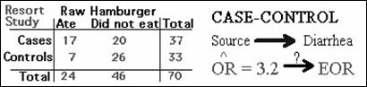
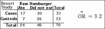
CASE-CONTROL STUDIES

Large-sample (Z or Chi Square) Test

This activity basically states chi-square approach can be used for case-control studies (including the MH chi–square) or one could use a Z statistic approach. From a practical perspective, most computer programs with provide chi-square results.

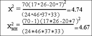
chi-square p-value: two-sided .030 one-sided .015

MH chi-square p-value two-sided .031 one-sided .015

Fisher exact two-sided .043 one-sided .026

Reject null - significant association between eating raw hamburger and illness.

Testing When Sample Sizes Are Small

Basically states that the Fisher exact test can be use with case-control data.

Large-Sample Confidence Interval

Description of how to calculate a 95% confidence interval for an odds ratio.

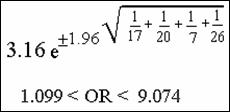
Study Question (12.16)

1. What interpretation can you give to this confidence interval?

Does not include null; “truth” is likely between 1.1 and 9.1

Calculating Sample Size for Case-Control and Cross-Sectional Studies

Will not ask questions concerning sample sizes on an exam.

COHORT STUDIES INVOLVING RATE RATIOS

Testing for Rate Ratios

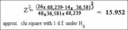
Statistical test applied to incidence density ratio data

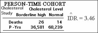
Chi-square approach

2-sided p-value < .001; 1-sided p-value < .01

Reject null hypothesis, conclude that those with borderline high cholesterol levels have a significantly higher mortality rate than those with normal cholesterol levels.

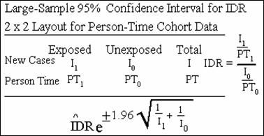
Large-Sample Confidence Interval (CI) for a Rate Ratio

Confidence interval for an incidence density ratio (IDR):

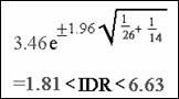
Study Question (12.19)

1. Interpret these results above. What do they mean?

We are 95% confident that “truth” is captured 1.81 and 6.63; does not include null value.

Quiz (12.20) Do not worry about these questions