LESSON 14 (Part 2)
![]()
Stratified Analysis
14-4 Stratified
Analysis
Precision-Based Adjusted Odds Ratio
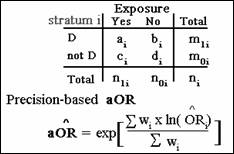
Thus far we have considered stratified data only from cohort studies
where the adjusted measure of effect is a precision-based risk ratio (aRR).
We now describe how to compute a precision-based adjusted odds ratio (aOR)
for stratified data from either case-control, cross-sectional, or cohort
studies in which the odds ratio is the effect measure of interest. Consider a general two-way data layout for
one of several strata. The
precision-based adjusted odds ratio is the exponential of a weighted average of
the natural log of the stratum-specific odds ratios. This formula applies
whether the study design used calls for the risk odds ratio, the exposure
odds ratio, or the prevalence odds ratio:
Below is the formula for the weights, which is
different for the adjusted odds ratio than for the adjusted risk ratio, because
precision is computed differently for different effect measures.
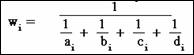
Let's focus on the weights for the adjusted
odds ratio. If all the cell frequencies for a given stratum are reasonably
large, then the denominator will be small, so its reciprocal, which gives the
precision, will be relatively large.
On the other hand, if one of the cell
frequencies is very small, the precision will tend to be relatively small. This
explains, at least for the odds ratio, why an unbalanced stratum with at least
one small cell frequency is likely to yield a relatively small weight even if
the total stratum size is large.

Summary
v The measure of association
used to assess confounding will depend on the study design.
v The formula for the adjusted
risk ratio applies when the study design used calls for the prevalence ratio
v The formula for the adjusted
odds ratio applies whether the study design used calls for the risk odds ratio,
the exposure odds ratio, or prevalence odds ratio.
v The weights are computed
differently for the adjusted odds ratio than for the adjusted risk ratio.
v An unbalanced stratum with at
least one small cell frequency is likely to yield a relatively small weight
even if the total stratum size is large.
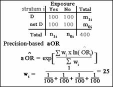
Computing the
Adjusted OR – An Example
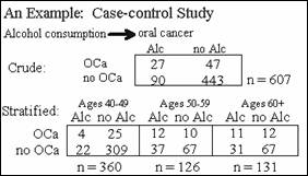
These tables show results from a case-control study to assess the
relationship of alcohol consumption to oral cancer. The tables give the crude
data when age is ignored and the stratified data when age has been categorized
into three groups.
Below is the
formula for the adjusted odds ratio for these data. Now, given that the weights for each strata
are as follows:
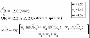
1.
What is the estimated adjusted odds ratio for these data? (Hint: Try to
answer without calculations.)
|
2.1 |
|
2.3 |
|
1.9 |
The estimated odds
ratio is 2.1.
2.
Are the crude and adjusted estimates meaningfully different?
|
yes |
|
no |
Yes, the crude
ratio of 2.8 indicates there is almost a three-fold excess risk but the
adjusted estimate of 2.1 indicates approximately a two-fold excess risk.
3.
Which estimate is more appropriate, the crude or the adjusted estimate?
|
crude |
|
adjusted |
The adjusted
estimate is more appropriate because it is meaningfully different from the
crude estimate and controls for the confounding due to age.
Quiz (Q14.11)
The data below are from a cross-sectional
seroprevalence survey of HIV among prostitutes in relation to IV drug use. The crude prevalence odds ratio is 3.59. (You may wish to use a calculator to answer
the following questions.)
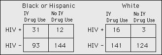
1.
What is the estimated POR among the Black or Hispanic
group? . . . . . ???
2.
What is the estimated POR among the Whites? . . . . . .
???
3.
Which table do you think is more balanced and thus
will yield the highest precision-based weight? . ???
Choices
3.25 3.59 4.00 4.31 4.69 Black or Hispanic White
In the study described in the previous question, the
estimated POR for the Black or Hispanic group was 4.00 and the estimated POR
for the Whites was 4.69. The precision-based weight for the Black or Hispanic
group is calculated to be 7.503 and the weight for the whites is 2.433.
4.
Using the formula below, calculate the adjusted POR
for this study. . . . . . ???
5.
Recall that the crude POR was 3.59. Does this provide
evidence of confounding? . . . ???
Choices
1.00 4.16 4.35 4.97 debatable no yes
14-5 Stratified
Analysis (continued)
Mantel-Haenszel Adjusted Estimates
The Zero-Cell
Problem
Let's consider the following set of results that might have occurred in
a case control study relating an exposure variable E to a disease D:
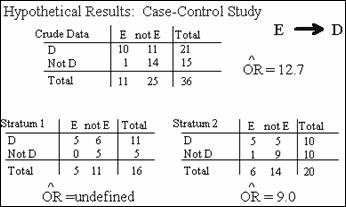
The odds ratio for
stratum 1 is undefined because
of the zero cell frequency in this stratum. So we cannot say whether there is
either confounding or interaction within these data. One approach sometimes taken to resolve such
a problem is to add a small number, usually .5, to each cell of any table with
a zero cell. If we add .5 here, the odds
ratio for this modified table is 9.3.
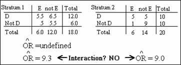
Now it appears that there is little evidence
of interaction since the two stratum-specific odds ratios are very close. But,
there is evidence of some confounding because the crude odds ratio is somewhat
higher than either stratum specific odds ratios. Although this approach to the zero-cell
problem is reasonable, and is often used, we might be concerned that the choice
of .5 is arbitrary.
Study Questions (Q14.12)
1.
Given the values a = 5, b = 6, c = 0, and d = 5 for stratum 1, what is
the estimated odds ratio if 0.1 is added to each cell frequency?
2.
Given the values a = 5, b = 6, c = 0, and d = 5 for stratum 1, what is
the estimated odds ratio if 1.0 is added to each cell frequency?
3.
What do your answers to the above questions say about the use of adding
a small number to all cells in a stratum containing a zero cell frequency?
We might also be concerned about computing a
precision-based adjusted odds ratio that involves a questionably modified
stratum-specific odds ratio.
Study Questions (Q14.12) continued
The
stratum-specific odds ratios obtained with .5 is added to stratum 1 are 9.31
for stratum 1 and 9.00 for stratum 2.
4.
If a precision-based adjusted odds ratio is computed by adding .5 to
each cell frequency in stratum 1 the weights are .3972 for stratum 1 and .6618
for stratum 2. What value do you obtain
for the estimated aOR?
The stratum-specific odds ratios obtained with
.1 is added to stratum 1 are 41.64 for stratum 1 and 9.00 for stratum 2.
5.
If a precision-based adjusted odds ratio is computed by adding .1 to
each cell frequency in stratum 1 the weights are .0947 for stratum 1 and .6618
for stratum 2. What value do you obtain
for the estimated aOR?
6.
How do your answers to the previous two questions compare?
7.
What do your answers to the previous questions say about the use of a
precision-based adjusted odds ratio?
Fortunately, there is an alternative form of
adjusted estimate to deal with the zero-cell problem called the Mantel-Haenszel
odds ratio, which we describe in the next activity.
Summary
v When there are sparse data in
some strata, particularly zero cells, stratum-specific odds ratios become
unreliable and possibly undefined.
v One approach when there are
zero cell frequencies in a stratum is to add a small number, typically 0.5, to
each cell frequency in the stratum.
v A drawback to the latter
approach is that the resulting modified stratum-specific effect estimate may
radically change depending on the small number (e.g., .5, .1) that is added.
v The use of a precision-based
adjusted estimate in such a situation then becomes problematic.
v Fortunately, there is an
alternative approach to the zero-cell problem, which involves using what is
called a Mantel-Haenszel adjusted estimate.
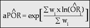
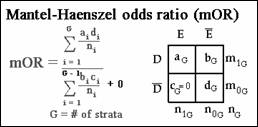
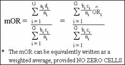
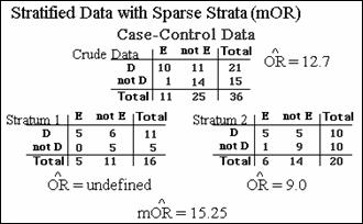
The Mantel-Haenszel Odds Ratio
The Mantel-Haenszel adjusted estimate used in case-control
studies is called the Mantel-Haenszel odds ratio, or the mOR.
Here is its formula:
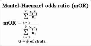
This formula can also be used to compute an
adjusted odds ratio in cross-sectional and cohort studies. A key feature of the mOR
is that it can be used without having to modify any stratum that contains a
zero-cell frequency. For example, if there is a
zero-cell frequency as shown below for the c-cell, then the computation
simply includes a zero in a sum in the denominator of the mOR, but the
total sum will not necessarily be zero.
Study Questions (Q14.13)
1.
Suppose there are G=5 strata and that either the b-cell or c-cell
is zero in each and every strata. What
will happen if you compute the mOR for these data?
2.
Suppose there are G=5 strata and that either the a-cell or d-cell
is zero in each and every strata. What
will happen if you compute the mOR for these data?
3.
What do your answers to the above questions say about using the mOR when
there are zero cell frequencies?
Another nice feature of the mOR is
that, even though it doesn't look it, the mOR can be written as a
weighted average of stratum-specific odds ratios provided there are no zero
cells in any strata. So the mOR will give a value somewhere between the
minimum and maximum-specific odds ratios over all strata, as will any weighted
average.
Still another feature of the mOR is
that it equals 1 only when the Mantel-Haenszel chi square statistic equals
zero. It is possible for the
precision-based aOR to be different from 1 even if the Mantel-Haenszel chi
square statistic is exactly equal to zero.
In general, the mOR has been shown to have good statistical
properties, particularly when used with matched case-control data. So it is
often used instead of the precision-based aOR even when there are no
zero-cells or the data are not sparse.
We now apply the mOR formula to the stratified
data example we have previously considered.
Substituting the cell-frequencies from each stratum into the mOR
formula, the estimated mOR turns out to be 15.25:
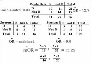
This adjusted estimate is somewhat higher than
the crude odds ratio of 12.7 and much higher than the odds ratio of 9.0 in
stratum 2. Because stratum 1 has an undefined odds ratio, we cannot say whether
there is evidence of interaction. However, because the crude and adjusted odds
ratios differ, there is evidence of confounding.
Study Questions (Q14.13) continued
If a precision-based adjusted odds ratio is computed by adding .5 to
each cell in stratum 1, the aOR that is obtained is 9.11. If, instead, .1 is added to each cell
frequency in stratum 1, the aOR is 10.65.
4.
Compare the aOR results above with the previously obtained mOR of
15.25. Which estimate do you prefer?
Summary
v For case-control studies as
well as other studies involving the odds ratio, an alternative to a
precision-based adjusted odds ratio is the Mantel-Haenszel odds ratio (mOR)
v Corresponding to the mOR, the
mRR or mIDR can be used in cohort studies.
v A key feature of the mOR is
that it may be used without modification when there are zero cells in some of
the strata.
v The mOR can also be written
as a weighted average of stratum-specific odds ratios provided there are
no zero cells in any strata.
v The mOR equals 1 only when
the Mantel-Haenszel chi square statistic equals zero.
v The mOR has been shown to
have good statistical properties, particularly when used with matched
case-control data.
Quiz (Q14.14)

True or False
1.
The practice of adding a small number to each of the
cells of a two by two table to eliminate a zero cell is arbitrary and should be
used with caution. . .
. . . . ???
2.
It is the adjusted estimate that is most affected by
adding a small number to each cell rather than the stratum specific estimates. . . . . . . . . ???
3.
When there are zero cell frequencies, the use of
Mantel-Haenszel adjusted estimates should be preferred since they can usually
be calculated without adjustment. . . . .
. ???
Interval Estimation
Interval Estimation - Introduction
We
now describe how to obtain a large-sample confidence interval around an
adjusted estimate obtained in a stratified analysis. This interval estimate can
take one of the two forms shown here:
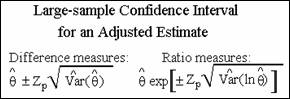
The Z in each expression denotes a
percentage point of the standard normal distribution. The θ
(“theta”) in each expression denotes the effect measure of interest. It can be
either a difference measure, such as risk difference, or a ratio measure, such
as a risk ratio. Typically, θ is a weighted average of stratum
specific effects. In particular, for risk difference measures, θ
will have a linear weighting as shown here:
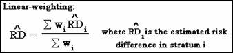
Mantel-Haenszel adjusted estimates for ratio
effect measures also have linear weighting.
For precision-based ratio estimates, θ
will have log-linear weighting.
The variance component within the confidence
interval will take on a specific mathematical form depending on the effect
measure. For precision-based measures, the variance component
conveniently simplifies into expressions that involve the sum of weights. In
particular, for precision-based difference measures, the confidence
interval formula reduces to form shown here:
For precision-based ratio measures, the
formula is written this way:

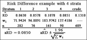
As an example, we again consider cohort data
involving four strata. We have four risk ratio estimates, their corresponding
precision-based weights and sample sizes, the crude risk ratio estimate, and
corresponding sample size.
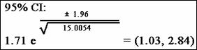
The adjusted risk ratio turns out to be 1.71.
To obtain the 95% precision-based interval estimate for this adjusted risk
ratio, we start with the formula shown here:
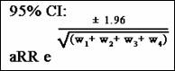
We
then substitute into the formula 1.71 for ![]() and the values shown in the table for the four weights:
and the values shown in the table for the four weights:
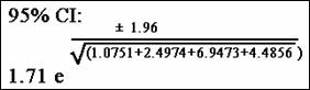
The lower and upper limits of the confidence
interval then turn out to be 1.03 and 2.84, respectively
Study Questions (Q14.15)
1.
How would you interpret the above confidence interval?
2.
Based on the information above, calculate a 95% confidence interval for
the adjusted risk difference. (You will
need to use a calculator to carry out this computation.)
3.
How do you interpret this confidence interval?
Summary
v A large-sample interval
estimate around an adjusted estimate can take one of the two forms:
![]() for difference effect
measures and
for difference effect
measures and
![]() for ratio effect measures
for ratio effect measures
v For risk difference measures
and for Mantel-Haenszel estimates, θ will have linear weighting.
v For precision-based ratio
estimates, θ will have log-linear weighting.
v For precision-based measures,
the variance component involves the sum of weights as follows:
 for difference
measures
for difference
measures
 for ratio measures
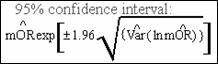
Interval Estimation for the mOR
Consider again the case-control stratified data involving sparse strata
that we previously used to compute a Mantel-Haenszel odds ratio. For
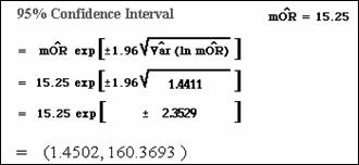
these data, the estimated Mantel-Haenszel odds ratio is 15.25.
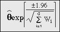
We find a 95% confidence interval around this
estimate with the formula shown here:
The variance term in this formula is a complex
expression involving the frequencies in each stratum. We present the variance
formula here primarily to show you how complex it is. Use a computer program to
do the actual calculations, which we will do for you here.
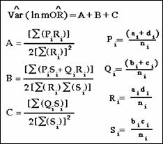
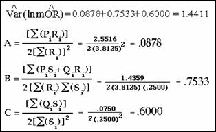
Substituting the frequencies in each stratum
into the formulae for Pi, Qi, Ri,
and Si, we obtain the values below. The estimated variance is shown here:
The 95% confidence interval is shown
below. Although this interval does not
contain the null value of 1, it is nevertheless extremely wide, which should
not be surprising given the sparse strata.
Summary
v A 95% confidence interval
around a Mantel-Haenszel odds ratio is given by the formula:
![]()
v The variance term in this
formula is a complex expression involving the frequencies in each stratum.
v You should use a computer to
calculate the variance term in the formula.
v You should not be surprised
to find a very wide confidence interval if all strata are sparse.
Quiz (Q14.16)
A case-control study was conducted to determine the
relationship between smoking and lung cancer. The data were stratified into 3
age categories. The results were: aOR = 4.51, and the sum of the weights =
3.44.
1.
Calculate a precision based 95% confidence interval
for these data.. . . . ???
2.
Do these results provide significant evidence that
smoking is related to lung cancer when controlling for age? . . . . . . . . . . ???
Choices
1.25, 10.78 1.57, 12.98 no yes
14-6
Stratified Analysis (continued)
Extensions to More Than 2 Exposure Categories
2xC Tables
A natural extension of stratified analysis for 2x2 tables
occurs when there are more than two categories of exposure. In such a case, the
basic data layout is in the form of a 2xC table where C denotes the number of
exposure categories. We now provide an overview of how to analyze stratified
2xC tables.
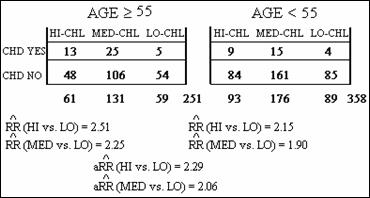
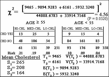
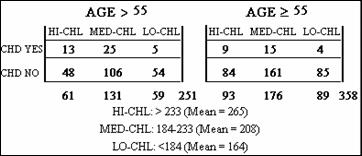
The tables shown here give the cholesterol level and the coronary heart
disease status for 609 white males within two age categories from a 10-year cohort
study in Evans County Georgia from 1960 to 1969.
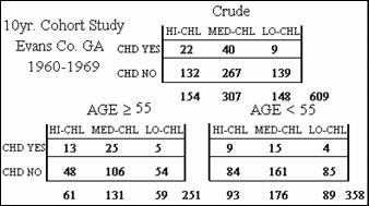
These data show three rather than two
categories of exposure for each of the two strata. How do we carry out a
stratified analysis of such data? We
typically carry out stratum-specific analyses and overall assessment, if
appropriate, of the exposure-disease relationship over all strata. But because there are three exposure
categories, we may wonder how to compute the multiplicity of effect measures
possible for each table, how to summarize such information over all strata, and
how to modify the hypothesis testing procedure for more than 2 categories.
Typically we compute several effect measures,
each of which compares one of the exposure categories to a referent exposure
category. In general, if there are C
categories of exposure, the basic data layout is a 2xC table. The
typical analysis then produces C-1 adjusted estimates, comparing C-1
exposure categories to the referent category.
Adjusted Estimates:
|
In our example, we will designate low
cholesterol to be the referent category. Because we have
cumulative-incidence cohort data, we compute two risk ratios per stratum, one
comparing the High Cholesterol category to the Low Cholesterol
Category and the other comparing the Medium Cholesterol category to the Low
Cholesterol category. Below are these estimates for each age group, and
precision-based adjusted estimates over both age groups. These results indicate a slight dose-response
effect of cholesterol on CHD risk. That is, the effect, as measured by the risk
ratio, decreases as the index group changes from high cholesterol to medium
cholesterol, when each group is compared to the low cholesterol group.
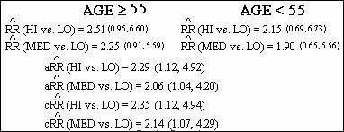
95% confidence intervals for both stratum
specific and adjusted odds ratios are shown below. The intervals for adjusted
risk ratios are obtained using the previously described formula involving the
sum of the weights.
Study Questions (Q14.17)
1.
Based on the information provided above, is there evidence that age is
an effect modifier of the relationship between cholesterol level and CHD risk?
2.
Based on your answer to the previous question, is it appropriate to carry
out overall assessment in this stratified analysis?
3.
Is there evidence of confounding due to age?
Summary
v When there are more than two
categories of exposure, the basic data layout is in the form of a 2xC
table where C denotes the number of exposure categories.
v As with stratified 2x2
tables, the goal of overall assessment is an overall adjusted estimate, and
overall test of hypothesis, and an interval estimate around the adjusted
estimate.
v When there are C
exposure categories, the typical analysis produces C=1 adjusted
estimates, which compare C-1 exposure categories to a referent category.
Test for Trend
We now describe how to test hypotheses for stratified data with several
exposure categories. We again consider the Evans County data shown here relating
cholesterol level to the development of coronary heart disease stratified by
age.
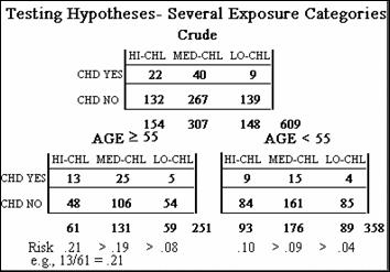
The exposure variable, cholesterol level, has
been categorized into three ordered categories. We can see that, for each
stratum, the CHD risk decreases as the cholesterol level decreases.
To see whether these stratum specific results
are statistically significant, we must perform a test for trend. Such a
test allows us to evaluate whether or not there is a significant dose-response
relationship between the exposure variable and the health outcome. The test for trend can be performed using an extension
of the Mantel-Haenszel test procedure. This test requires that a numeric
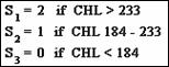
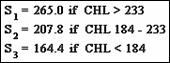
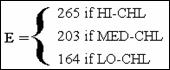
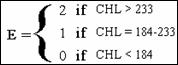
value or score be assigned to each category of exposure. For example, the three ordered categories of
exposure could be assigned scores of 2 when cholesterol is greater than 233, 1
when cholesterol is between 184 and 233, and 0 if cholesterol is below 184.
Alternatively, the scores might be determined
by the mean cholesterol value in each of the ordered categories. For these
data, then, the scores turn out to be 265.0, 207.8 and 164.4 for the high,
medium, and low cholesterol categories, respectively.
The general formula for the test statistic is
shown here:
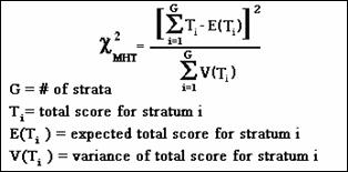
The number of strata is G. Typically
this formula should be calculated using a computer. In our example, there are
two age strata, so G=2. The trend test formula then simplifies as shown here (the
box at the end of this activity shows how to perform the calculations):
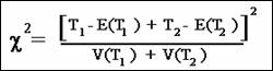
We will use this simplified formula to compute
the test for trend where we will use as our scores rounded, mean-cholesterol
values for each cholesterol category. Here are the results:
Study Questions (Q14.18)
1.
Give two equivalent ways to state the null hypothesis for the trend test
in this example.
2.
Based on the results for the trend test, what do you conclude?
3.
If a different scoring method was used, what do you think would be the
results of the trend test?
Let's see what the chi square results would be
when we use a different scoring system. Here are the results when we use 2, 1,
and 0.
Study Questions (Q14.18) continued
4.
How do the results based on 2, 1, 0 scoring compare to the results based
on 265, 208, 164?
5.
What might you expect for the trend test results if the scoring was 3,
2, 1 instead of 2, 1, 0?
Summary
v If the exposure variable is
ordinal, a one d.f. chi square test for linear trend can be performed using an
extension of the Mantel-Haenszel test procedure.
v Such a “trend” test can be
used to evaluate whether or not there is a linear dose-response relationship of
exposure to disease risk.
v To perform the test for
trend, a numeric value or score must be assigned to each category of exposure.
v The null hypothesis is that
the risk for the health outcome is the same for each exposure category.
v The alternative hypothesis is
that the risk for the health outcome either increases or decreases as exposure
level increases.
v The test statistic is best
calculated using a computer.
Testing for Overall Association
Using Logistic Regression
The test for trend that we described in the previous activity can
alternatively be carried out using a logistic regression model. Here again is the logistic model and its
equivalent logit form as defined in an earlier lesson:
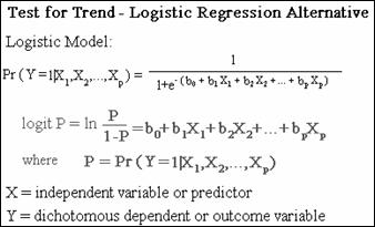
The X's in the model are the independent
variables or predictors; Y is the dichotomous dependent
or outcome variable, indicating whether or not a person develops the
disease. We now describe the specific
form of this model for the previously considered Evans County data, relating
three categories of cholesterol to the development of CHD within 2 age
categories. These data are shown again here:
The logistic model appropriate for the trend
test for these data takes the following logit form:
![]()
The E variable in this model represents
cholesterol. The A variable represents age. More specifically, E
is an ordinal variable that assigns scores to the three categories of exposure.
The scores can be defined as the mean cholesterol value in each cholesterol
category:
If the scores are instead, 2, 1, and 0, then
we define the E variable as shown here:
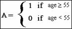
The A variable is called a dummy
or indicator variable; it distinguishes the two age strata being
considered:
Study Questions (Q14.19)
In general, if there are S
strata, then S – 1 dummy variables are required. For example, if there were 3 strata, then 2
dummy variables are required. One way to
define the 2 variables would be:
A1 = 1 if stratum
1, else 0, A2 = 1 if stratum 2, else 0
For such coding:
A1 = 1, A2 = 0 for stratum 1
A1 = 0, A2 = 1 for stratum 2
A1 = 0, A2 = 0 for stratum 3
Using such coding, stratum 3 is called the referent
group.
Suppose we wanted
to stratify by two categories of age (e.g., 1 = Age > 55 vs. 0 = Age
< 55) and by gender (1 = females, 0 = males).
1.
How many dummy variables would you need to define?
2.
How would you define the dummy variables (e.g., D1, D2, etc.) if the
referent group involved males under 55 years old?
3.
Define the logit form of the logistic model that would incorporate this
situation and allow for a trend test the uses mean cholesterol values as the
scores.
For the model involving only 2 age strata, the
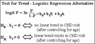
null hypothesis for the test for trend is that the true coefficient of the
exposure variable, E, is zero. This is equivalent to saying there is no linear
trend in the CHD risk, after controlling for age. The alternative hypothesis is
that there is a linear trend in the CHD risk, after controlling for age.
We use a computer program to fit the logistic
model to the Evans County data. When we define the E variable from the
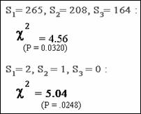
mean cholesterol in each exposure category, a chi square statistic that tests
this null hypothesis has the value 4.56.
This statistic is called the Likelihood
Ratio statistic and it is approximately a chi square with 1 d.f. The
P-value for this test turns out to be 0.0327. Because the P-value is less than
.05, we reject the null hypothesis at the 5% significance level and conclude
that there is significant linear trend in these data.
Study Questions (Q14.19) continued
When
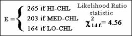
exposure scores are assigned to be 2, 1, and 0 for HI-CHL, MED-CHL, and LO-CHL,
respectively, the corresponding Likelihood Ratio test for the test for trend
using logistic modeling yields a chi square value of 5.09 (P = .0240).
4.
How do these results compare with the results obtained using mean
cholesterol scores? (chi square = 4.56, P = .0327)
When computing the test for trend in the
previous activity (using a summation formula), the results were as follows:
Mean cholesterol scores: chi square = 4.60 (P = .0320)
2, 1, 0 scores: chi square = 5.04 (P = .0248)
5.
Why do you think these latter chi square results are different from the
results obtained from using logistic regression? Should this worry you?
Summary
v Testing hypothesis involving
several categories of exposure can be carried out using logistic regression.
v If the exposure is nominal,
the logistic model requires dummy variables to distinguish exposure categories.
v If the exposure is ordinal,
the logistic model involves a linear term that assigns scores to exposure
categories.
v For either nominal or ordinal
exposure variables, the test involved a 1 d.f. chi square statistic.
v The null hypothesis is no
overall association between exposure and disease controlling for stratified
covariates.
v Equivalently, the null
hypothesis is the coefficient of the exposure variable in the model is zero.
v
The test can be performed using either a likelihood ratio test or a Wald
test, which usually give similar answers, though not always.
Quiz (Q14.20)
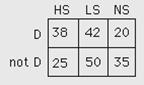
The data to the right are from a case-control study
conducted to investigate the possible association between cigarette smoking and
myocardial infarction (MI). All subjects were white males between the ages of
50 and 54. Current cigarette smoking practice was divided into three
categories: nonsmokers (NS), light smokers (LS), who smoke a pack or less each
day, and heavy smokers (HS), who smoke more than a pack per day.
1.
What is the odds ratio for HS vs. NS? ???
2.
What is the odds ratio for LS vs. NS? ???
Choices
1.47 1.78 2.66 2.70 3.06
All subjects were categorized as having "high" or
"low" social status (SS) according to their occupation, education,
and income. The stratum-specific data are shown below.
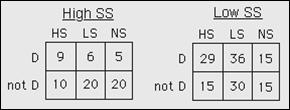 Quiz
continued on next page
Quiz
continued on next page
3.
Calculate the stratum specific odds ratios:
a.
High SS: HS vs. NS ???
b.
High SS: LS vs. NS ???
c.
Low SS: HS vs. NS ???
d.
Low SS: LS vs. NS ???
4.
Is it appropriate to conduct an overall assessment for
these data? ???
Choices
0.01 1.20 1.93 3.50 3.60 5.40 maybe no yes
Consider the following results:
Crude OR, HS vs. NS = 2.66
Crude OR, LS vs. NS = 1.47
Adjusted OR, HS vs. NS = 2.38
Adjusted OR, LS vs. NS = 1.20
5.
Do these results provide evidence of trend? ???
Choices
no yes
The Mantel-Haenszel test for trend was performed using
scores of 0, 1, 2 for nonsmokers, light smokers, and heavy smokers,
respectively. The Mantel-Haenszel Chi-square statistic = 5.1. This corresponds
to a one-sided p-value of 0.012.
6.
What do you conclude at the 0.05 level of
significance? ???
7.
What do you conclude at the 0.01 level of
significance? ???
Choices
fail to reject H0 reject H0
8.
An alternative test for trend for these data can be
performed using a logistic model. Define the logit form of the logistic model
that would incorporate this situation and allow for a trend test. ???
Choices
Logit P = b0 + b1SMK + b2SES
Logit P = b0 + b1SMK + b2SES1
+ B3SES2
Logit P = b0 + b1SMK + b2SMK2
+ B3SMK3 + b4SES