LESSON 13
![]()
Options
for controlling for confounders
Design
options
Randomization
RCT only
Groups are similar (on both measured and unmeasured
factors)
Restriction
Easy, inexpensive
Generalizability
Matching – most freq with case-control
studies
Gain precision
Number of controls per case
Matched analyses
Analysis
options
Stratified analysis
Mathematical modeling
A mathematical model is a mathematical expression that describes
how an outcome variable can be predicted from explanatory variables.
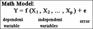
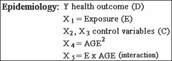
In epidemiology many times the outcome variable is dichotomous. When the
dependent variable is dichotomous, the most popular mathematical model is a
non-linear model called the logistic model.
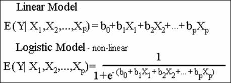
Table 14-2. Example Data 1:
Hypothetical cohort study of the relationship between smoking and coronary
heart disease (CHD) stratified on sex
Females
|
|
Smoker |
Non-Smoker |
|
|
CHD |
5 |
8 |
13 |
|
No
CHD |
45 |
142 |
187 |
|
|
50 |
150 |
200 |
|
Risk |
10.0% |
5.3% |
|
Odds Ratio for
females (ORf) = 2.0 (0.6, 6.3)
Males
|
|
Smoker |
Non-Smoker |
|
|
CHD |
300 |
50 |
350 |
|
No
CHD |
300 |
150 |
450 |
|
|
600 |
200 |
800 |
|
Risk |
50.0% |
25.0% |
|
Odds Ratio for
males (ORm) = 3.0 (2.1, 4.3)
----
Summary information
Directly
adjusted OR = 2.9 (2.1, 4.1)
Mantel-Haenszel OR = 2.9 (2.1, 4.1)
Chi-square
p-value (MH) p-value < .001
Table 14-9. Example data 1:
Hypothetical cohort study of the relationship between smoking and coronary
heart disease (CHD) controlling for the sex of the individual, logistic
regression model
There
were 363 type 1.0's
(model gives log odds of this type) and 637 type .0's.
Log
likelihood = -575.0730
Likelihood
ratio = 158.1036 2 df (P = .0000)
Dependent
Variable = CHD
Standard
Coefficient Error
Coef/SE "P value"
CONSTANT -3.0336
.2997 -10.1211 .0000
SMOKE 1.0618 .1733 6.1277 .0000
SEX 1.9643 .3045 6.4505
.0000
95.0-% confidence limits
Coefficient Odds ratio
lower upper lower upper
limit limit limit limit
SMOKE .7222
1.0618 1.4015 2.0590 2.8916 4.0611
SEX 1.3675
1.9643 2.5612 3.9254 7.1302
12.9513
TABLE
14-14. Advantages and disadvantages of
stratification and logistic regression.
|
|
Stratification |
Logistic Regression |
|
Parameters estimated |
RR,
RD, OR, IDR, IDD, others |
OR |
|
Validity of parameters
estimated |
More
valid (no model assumptions) |
Less
valid (based on model assumptions) |
|
Exposure and third
variables |
Must
be categorical |
Can
be categorical or continuous |
|
Number of third variables
or categories in third variables |
Compared
to logistic regression, limited |
Compared
to stratified analysis, can usually have many more variables or variables
with many categories |